30 Day Map Challenge 2024 - Day 5: A journey

On day five, the theme is A journey:

Map any journey. Personal or not. Trace a journey - this could be a daily commute, a long-distance trip, or something from history. The key is to map movement from one place to another.

Data

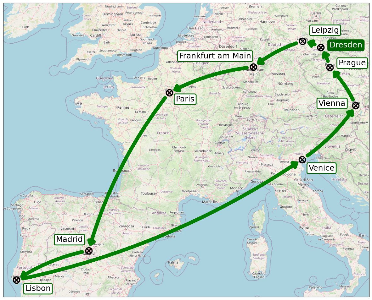
For today’s task, we need to compile a custom data set that cannot be found ready for use anywhere. I want to map the Grand Tour that Augustus II the Strong undertook from May 19th, 1687 to April 28th, 1689. On his journey, he was to get to know the architecture and culture of other countries, enhance his foreign language skills, learn manners and gain diplomatic skills and experience.

Starting in Dresden, his tour took him via Leipzig and Frankfurt am Main to Paris, where he spent a long time at the court of the “Sun King” Louis XIV. After a short detour to Madrid, he returned to Paris. From there, he traveled via Madrid and Lisbon to Venice and finally back to Dresden via Vienna and Prague. The details of the journey vary from source to source, but the overall route is roughly similar.

Implementation

The necessary imports include the usual mapping and data handling libraries. geopy provides an abstraction to convenientky access the Nominatim API that uses OpenStreetMap data to retrieve a city’s coordinates by name.

import cartopy.crs as ccrs
import cartopy.io.img_tiles as cimgt
import matplotlib.pyplot as plt
import pandas as pd
from geopy.geocoders import Nominatim
from matplotlib.patches import FancyArrowPatch

First, we have to get the location of each of the cities on the journey, store it in a pandas DataFrame. Additionally, we add two columns that hold the next destination, which makes drawing the connections much easier when creating the map.

geolocator = Nominatim(user_agent="30daymapchallenge")

df = pd.DataFrame(
    [
        {"city": city, "latitude": location.latitude, "longitude": location.longitude}
        for city in [
            "Dresden",
            "Leipzig",
            "Frankfurt am Main",
            "Paris",
            "Madrid",
            "Lisbon",
            "Venice",
            "Vienna",
            "Prague",
            "Dresden",
        ]
        if (location := geolocator.geocode(city)) is not None
    ]
).assign(
    dest_lat=lambda df: df["latitude"].shift(-1),
    dest_lon=lambda df: df["longitude"].shift(-1),
)

From the list of coordinates, we now have to extract the bounding box that defines the area the map should show. It’s compiled from the minimum and maximum value of latitude and longitude components, respectively. An additional margin of 1 degree in each direction prevents content laying directly on the border of the map.

bounds = [
    coord
    for coords in zip(
        df[["longitude", "latitude"]].min() - 1, df[["longitude", "latitude"]].max() + 1
    )
    for coord in coords
]

For a nice arrangement of the labels that contain each city’s name, we define a dictionary that holds offset values (in unit points), which will be used later when rendering annotations on the map.

offset_map = {
    "Dresden": (20, 0),
    "Leipzig": (20, 20),
    "Frankfurt am Main": (-170, 20),
    "Paris": (15, -20),
    "Madrid": (-75, 20),
    "Lisbon": (20, -25),
    "Venice": (15, -25),
    "Vienna": (-85, 0),
    "Prague": (20, 5),
}

Based on this data, we can now build the map visualizing the journey of August II the Strong. First, we set OpenStreetMap as the provider for background tiles and retrieve an axis object to work with.

Then we loop over all the cities in the dataframe, plot a marker at the specific location, as well as an annotation that prints the city’s name. Here, we use the offset mapping from above to shift the label accordingly.

Finally, if there is a succeeding destination for the current city, we plot a nice arrow that visualizes the direction of travel. For the offset of the annotations, as well as the shrinkA and shrinkB parameters of the FancyArrowPatch, it is important to note that those are in unit points. This is very useful for achieving the same distance on the map for equal values, which are not affected by the projection in use.

tiles = cimgt.OSM()

fig = plt.figure(figsize=(15, 15))
ax = fig.add_subplot(1, 1, 1, projection=tiles.crs)

ax.set_extent(bounds, crs=ccrs.Geodetic())

ax.add_image(tiles, 6)

for label, city in df.iterrows():
    ax.plot(
        city["longitude"],
        city["latitude"],
        marker=r"$\bigotimes$",
        color="black",
        markersize=16,
        transform=ccrs.Geodetic(),
    )

    ax.annotate(
        city["city"],
        xy=(city["longitude"], city["latitude"]),
        xycoords="data",
        xytext=offset_map[city["city"]],
        textcoords="offset points",
        fontsize=18,
        transform=ccrs.Geodetic(),
        color="white" if city["city"] == "Dresden" else "black",
        bbox=dict(
            boxstyle="round,pad=0.2",
            fc="darkgreen" if city["city"] == "Dresden" else "white",
            ec="darkgreen",
            lw=2,
        ),
    )

    if city.isnull().any():
        continue

    arrow = FancyArrowPatch(
        (city["longitude"], city["latitude"]),
        (city["dest_lon"], city["dest_lat"]),
        connectionstyle="arc3,rad=.1",
        arrowstyle="Simple, head_width=12, head_length=8",
        color="green",
        shrinkA=15,
        shrinkB=15,
        lw=8,
    )
    patch = ax.add_patch(
        arrow,
    )
    patch.set_transform(ccrs.Geodetic())


plt.show()