30 Day Map Challenge 2024 - Day 4: Hexagons
On day four, the theme is Hexagons:
Maps using hexagonal grids. Step away from square grids and try mapping with hexagons. A fun way to show density or spatial patterns.
Data
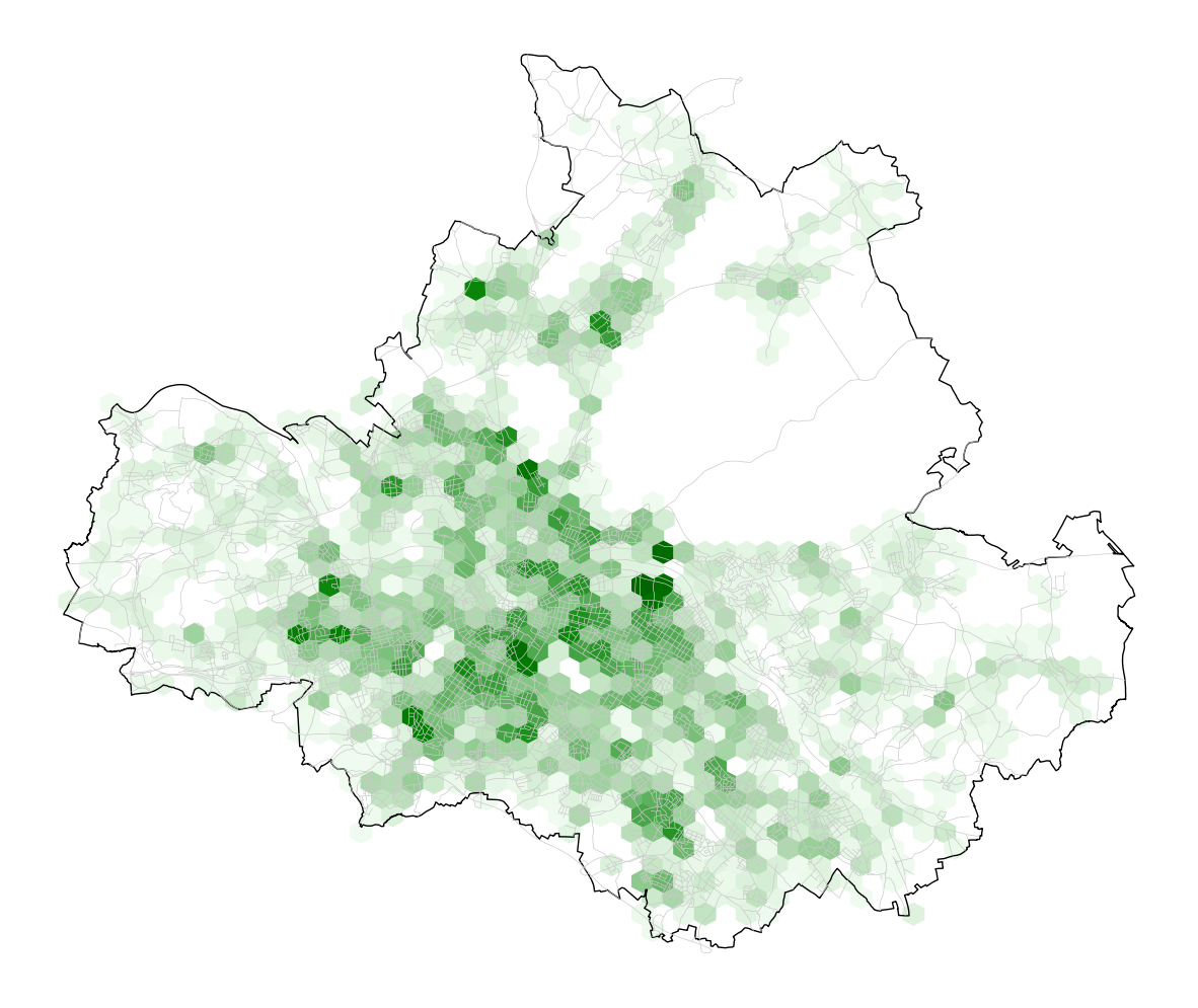
The idea for today is building a heatmap that visualizes the tree-density in the city. This does not include natural structures, like forests and parks. Therefore, the map shows hardly any tree on the area of Dresden Heath, which is one of the largest municipal forests in Germany.
The OpenDataPortal gives the following explanation of the data set (translation by me):
Dresden is a city rich in trees with a great diversity of species. Avenues and valuable trees in the parks, green spaces and gardens characterise the cityscape. Trees make a significant contribution to the quality of life as they have a positive influence on the urban climate. There are currently around 98,700 registered trees in urban areas. These include street trees, trees in parks and green spaces, on playgrounds, on open spaces of educational institutions, along waterways of the 2nd order and on other municipal areas.
In addition to the widely represented typical tree species such as lime, maple and chestnut, over 139 species and varieties of ginkgo, magnolia, leather tree and other rarer tree species grow in the urban area.
Implementation
As always, some imports are required.
Today, we create a static plot using matplotlib.
For the definition of the read_dresden_csv function, see the post for day 2.
1
2
3
4
import matplotlib.pyplot as plt
import matplotlib.colors as clrs

from utils import read_dresden_csv
Besides the data for background information (city boundary, and streets), we load the actual tree data set for today. Right after loading the data, we split the coordinates into latitude and longitude components, which simplifies the calculation of hexbins later. With this, we get 116,751 records, i.e. tree locations:
1
2
3
4
5
gdf_trees = read_dresden_csv("data/dresden/stadtbaeume.csv", geometry_column="geom")
gdf_trees[['longitude', 'latitude']] = gdf_trees.get_coordinates()

gdf_city_boundary = read_dresden_csv("data/dresden/city_boundary.csv", geometry_column="shape")
gdf_streets = read_dresden_csv("data/dresden/verkehrswege.csv", geometry_column="shape")
For visualization, we first create a figure and axis object using matplotlib and define some colors, as well as a colorbar for the heatmap.
Matplotlib already provides a function for binning and plotting data using hexagons.
We just need to provide the data, define the resolution (gridsize) and set the colorbar.
The parameter setting for vmin=1 is very important for the colorbar to start at 1 and not 0.
This way, hexbins that are empty get an alpha value of 0 (cmap.set_under(alpha=0)) and therefore are fully transparent.
1
2
3
4
5
6
7
8
9
10
11
12
13
14
15
16
17
18
19
20
21
22
23
fig, ax = plt.subplots(1, 1, figsize=(15, 15))
background_color = "#ffffff"
street_color = "#cacaca"
boundary_color = "black"
ax.set_facecolor(background_color)
ax.axis("off")  # remove frame and axis ticks

cmap = clrs.LinearSegmentedColormap.from_list("", ["#effbef","green","darkgreen"])
cmap.set_under(alpha=0)

gridsize = 50
plt.hexbin(
    x=gdf_trees['longitude'],
    y=gdf_trees['latitude'],
    gridsize=(gridsize, gridsize//2),
    cmap=cmap,
    vmin=1,  # 0 trees should be considered "under" for correct alpha value
)

gdf_streets["shape"].plot(color=street_color, ax=ax, linewidth=.5)
gdf_city_boundary["shape"].plot(edgecolor=boundary_color, facecolor="none", ax=ax)

plt.show()