30 Day Map Challenge 2024 - Day 2: Lines
The theme of the second day is Lines:
A map with focus on lines. Roads, rivers, routes, or borders - this day is all about mapping connections and divisions. Another traditional way to keep things moving.
Data
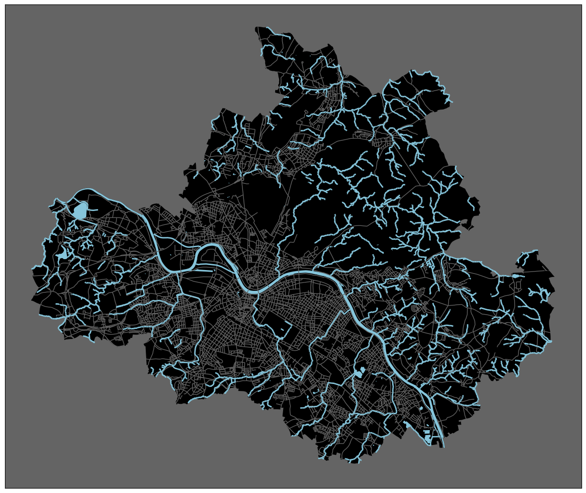
Again, I will select data from the Dresden OpenDataPortal to visualize. Specifically, I want to create a map of all standing and flowing waters in the city of Dresden. The most prominent one here is the Elbe, a major river in Europe, which flows from east to west and divides the city in two parts. Obviously, the northern part of the city is the better one! The Elbe’s source lays in the Giant Mountains of the northern Czech Republic. After 1094 km, it flows into the North Sea at Cuxhaven (northwest of Hamburg).
For today’s visualization, I downloaded five datasets. While the first three serve the main purpose of mapping standing and flowing waters, the latter two will provide some background information that improve orientation.
Implementation
First, we need of course to import required libraries and load the data for today.
1
2
3
4
from pathlib import Path
import geopandas as gpd
import pandas as pd
import matplotlib.pyplot as plt
Since we need to load several CSV files today, I first create a method that performs file reading and transformation into a GeoDataFrame in one go.
This way, we can easily call the method on different files, which makes loading data much more convenient.
Later on, I will copy this method into its own file, so I can import and reuse it on other days again.
1
2
3
4
5
6
7
8
9
10
def read_dresden_csv(file_path: str | Path, geometry_column: str, srid: int=4326) -> gpd.GeoDataFrame:
    df = pd.read_csv(file_path, delimiter=";", header=0)
    df[geometry_column] = gpd.GeoSeries.from_wkt(
                df[geometry_column].str.removeprefix(f"SRID={srid};")
            )
    return gpd.GeoDataFrame(
        df,
        geometry=geometry_column,
        crs=f"EPSG:{srid}",
    )
Now, we can load today’s data sets:
1
2
3
4
5
6
gdf_rivers = read_dresden_csv("data/dresden/fliessgewaesser.csv", geometry_column="shape")
gdf_elbe = read_dresden_csv("data/dresden/elbe-stehende-gewaesser.csv", geometry_column="shape")
gdf_standing = read_dresden_csv("data/dresden/stehende-gewaesser.csv", geometry_column="shape")

gdf_city_boundary = read_dresden_csv("data/dresden/city_boundary.csv", geometry_column="shape")
gdf_streets = read_dresden_csv("data/dresden/verkehrswege.csv", geometry_column="shape")
Today, I will create a static, non-interactive plot:
1
2
3
4
5
6
7
8
9
10
11
12
13
14
15
16
17
18
fig, ax = plt.subplots(1, 1, figsize=(15,15))

background_color = "#646464"
water_color = "#86c5db"

ax.set_facecolor(background_color)

gdf_city_boundary["shape"].plot(color="black", ax=ax)
gdf_streets["shape"].plot(color=background_color, ax=ax, linewidth=1)

gdf_rivers["shape"].plot(ax=ax, color=water_color, linewidth=2)
gdf_elbe["shape"].plot(ax=ax, color=water_color)
gdf_standing["shape"].plot(ax=ax, color=water_color)

plt.xticks([])
plt.yticks([])

plt.show()